Bar plot in ggplot2

Euro Cup 2016

The group matches are not exciting to me. What excites me is the knock-out games! I started watching Euro Cup 2016 from quarter finals. Due to different time zone, we always have to stay awake almost all night to watch the game. I predicted Germany to win this Euro Cup, however they were defeated by France. All my friends were predicting France to win the final, and looking at the game, it was obvious France will win. France played brilliantly but they just couldn’t score a goal to take away the cup. I would say that night, lady luck was sitting on Portugal.

Apart from games, I was also interested in game statistics. I have waited for the tournament to get over so that I can see the final statistics.

Getting and Cleaning Data

The data is posted on official UEFA site. And to transfer the data table posted on the website to R, I have used rvest package.

library(rvest)

And to copy the data table from the site, the code goes like this

attempts <- read_html("http://www.uefa.com/uefaeuro/season=2016/statistics/round=2000448/teams/category=attacking/kind=attempts/index.html")

attemptsData <- attempts %>% 
  html_nodes("table") %>% 
  .[[1]] %>% 
  html_table()

First, we have to save the url page where the table is displayed. Then using rvest function html_nodes(“table”) and then .[[1]] for table 1 and then html_table(), we can easily copy the table. In fact, the page has only one table. If there were two tables and we wanted both then we would have used .[[2]] to transfer table number 2. For more detail, please read rvest package info.

Once the data is successfully transfered to R, we can do some data exploration like

str(attemptsData)
head(attemptsData)

While looking at the data, I have noticed that some unwanted characters appeared on the Team name column. In order to remove unwanted character, I have used base R function substr and str_trim from stringr package.

attemptsData$Name <- substr(attemptsData$Name, 6, 70)
attemptsData$Name <- str_trim(attemptsData$Name, side = "left")

substr function removed the first 5 unwanted characters and left with spaces on the left side. While the country/team names are on the right side, I have used str_trim(, side = “left”) to remove all the spaces on the left which also made other unwanted characters go.

Once the data is cleaned, I have saved the data in the local disk.

write.csv(attemptsData, "attempts.csv", row.names = FALSE)

Here is the glimpse of data -

head(attemptsData)

Name	Total.attempts	Attempts.per.game	On.target	Off.target	Blocked	Hit.woodwork
France	121	17.29	43	42	36	6
Wales	68	11.33	32	22	14	0
Portugal	121	17.29	39	49	33	3
Belgium	98	19.60	39	49	25	0
Iceland	40	8	19	16	5	1
Germany	108	18	37	46	25	4

tail(attemptsData)

Name	Total.attempts	Attempts.per.game	On.target	Off.target	Blocked	Hit.woodwork
Russia	34	11.33	6	17	11	0
Turkey	26	8.67	4	15	7	0
Albania	30	10.00	8	12	10	1
Austria	40	13.33	10	17	13	2
Sweden	23	7.67	3	12	8	0
Ukraine	43	14.33	13	19	11	0

The copied data after cleaning is hosted on this repo. Feel free to use it.

Visualization

Load the ggplot2 package.

library(ggplot2)

Basic Bar Plot

ggplot(attempts, aes(x = Name, y = Total.attempts)) +
  geom_bar(stat = "identity")

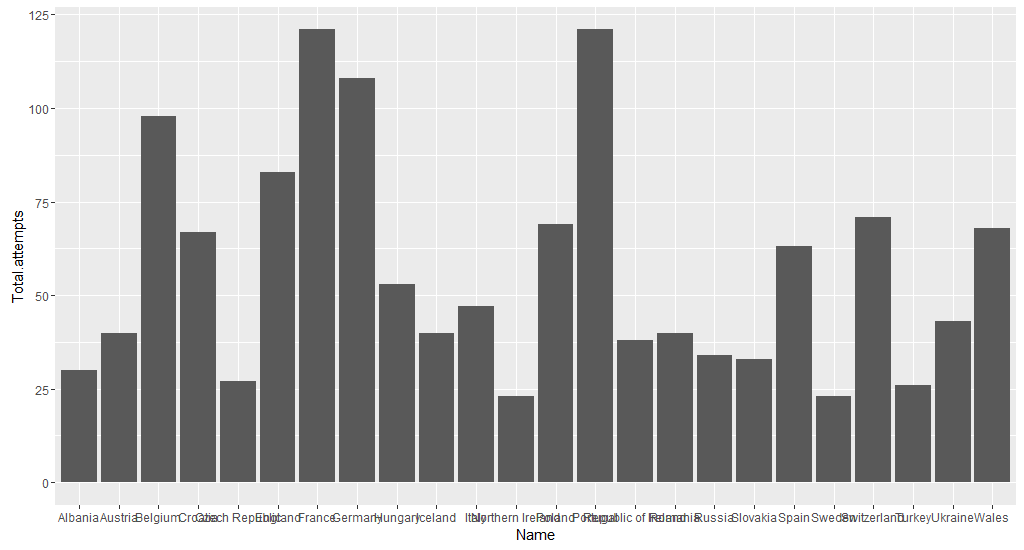
From the above ggplot, we can’t make out what’s in the x-axis. The y-label is not properly named. In order to read the x-axis well, I have flipped the ggplot. I have added ### to identify the new line of code.

ggplot(attempts, aes(x = Name, y = Total.attempts)) +
  geom_bar(stat = "identity") +
  coord_flip() ###

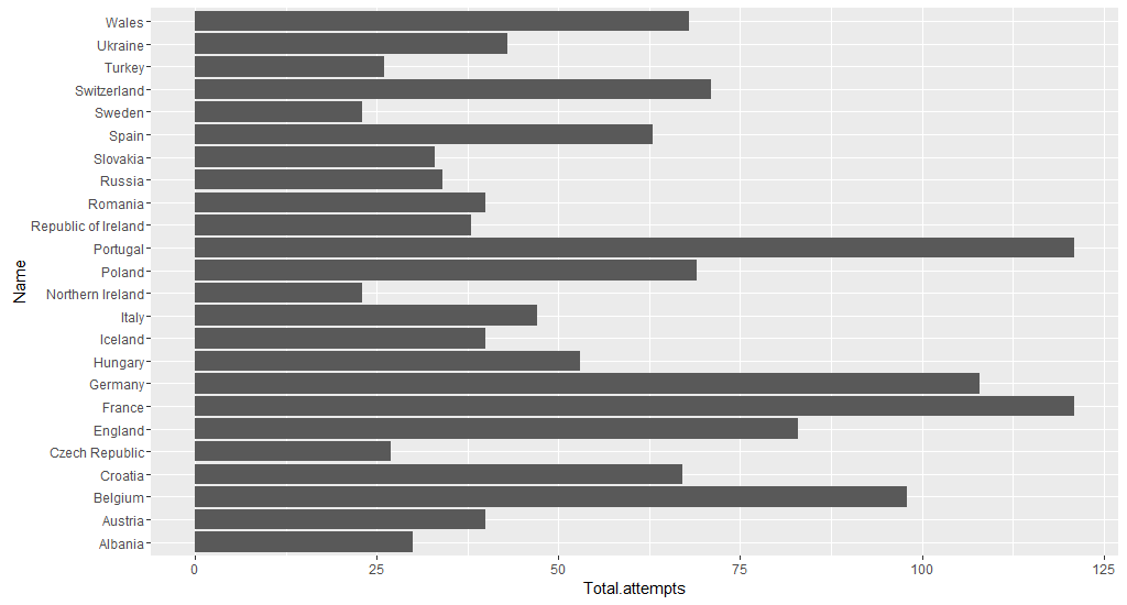
Now we can read the country/team names properly. I want to label the x-axis and y-axis appropriately. X-axis label name “Name”, I will keep it empty and y-axis label name to “Attempts”. Also, add title to the ggplot.

ggplot(attempts, aes(x = Name, y = Total.attempts)) +
  geom_bar(stat = "identity") +
  coord_flip() +
  ggtitle("Total Attempts by Team in EuroCup 2016") + ###
  labs(x = "", y = "Attempts") ###

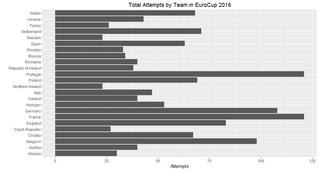
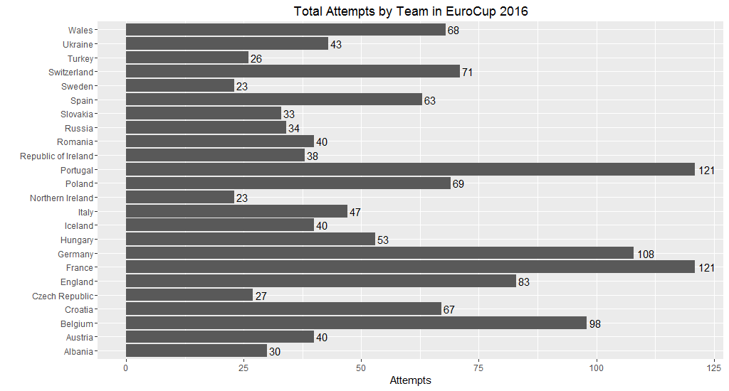
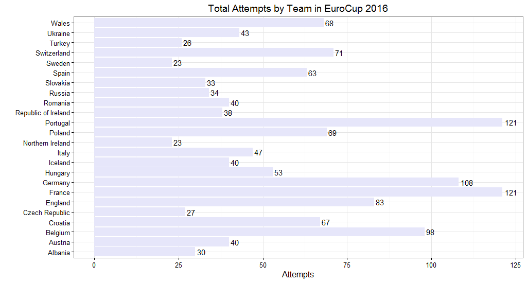
Now I want to display the attempts made by country/team on their respective bar.

ggplot(attempts, aes(x = Name, y = Total.attempts)) +
  geom_bar(stat = "identity") +
  geom_text(aes(label = Total.attempts), hjust = -0.2) + ###
  coord_flip() +
  ggtitle("Total Attempts by Team in EuroCup 2016") +
  labs(x = "", y = "Attempts")

Change the colour of bar and remove the grey background. To see the colours available in R, we can run colors() in the console and it will display all the colours name.

ggplot(attempts, aes(x = Name, y = Total.attempts)) +
  geom_bar(stat = "identity", fill = "lavender") + ###
  geom_text(aes(label = Total.attempts), hjust = -0.2) + 
  coord_flip() +
  ggtitle("Total Attempts by Team in EuroCup 2016") +
  labs(x = "", y = "Attempts") +
  theme_bw() ###

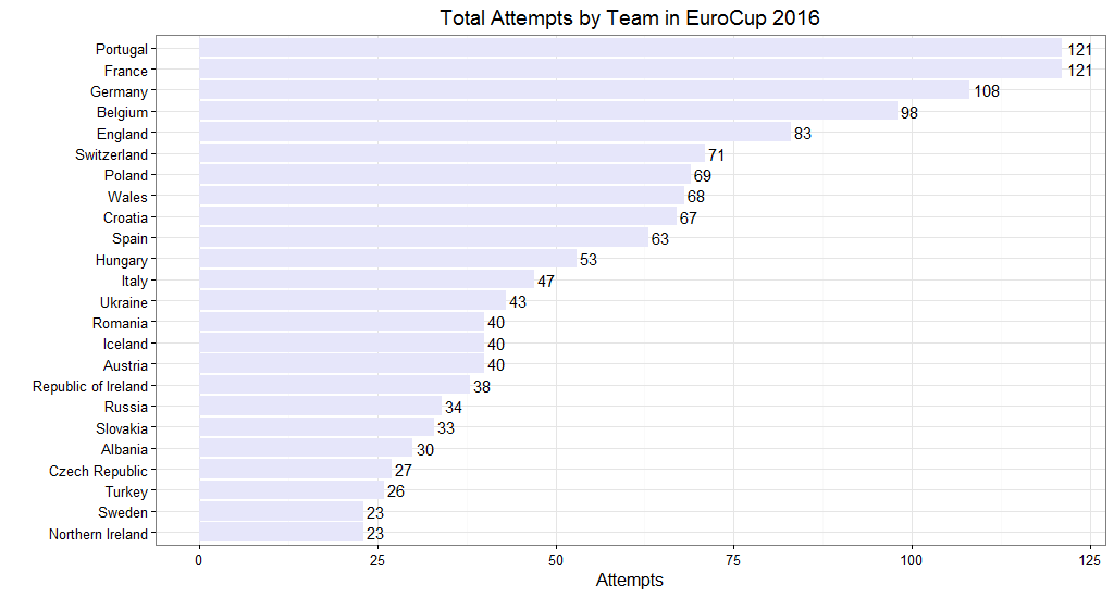
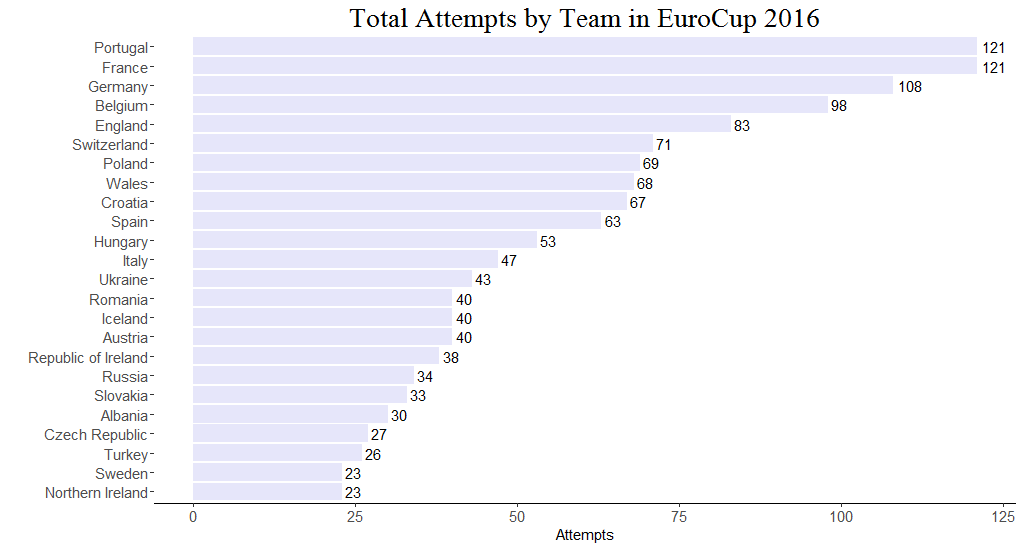
Let’s reorder the bar in descending order as per attempts made by country/team. For this we need to manipulate data little bit. We arrange the variable Total.attempts in descending order and also use reorder() in ggplot. For arranging Total.attempts in descending order, we will use dplyr package. We can also use base function order().

require(dplyr)
attempts <- arrange(attempts, desc(Total.attempts))

ggplot(attempts, aes(x = reorder(Name, Total.attempts), y = Total.attempts)) + ###
  geom_bar(stat = "identity", fill = "lavender") +
  geom_text(aes(label = Total.attempts), hjust = -0.2) +
  coord_flip() +
  ggtitle("Total Attempts by Team in EuroCup 2016") +
  labs(x = "", y = "Attempts") +
  theme_bw()

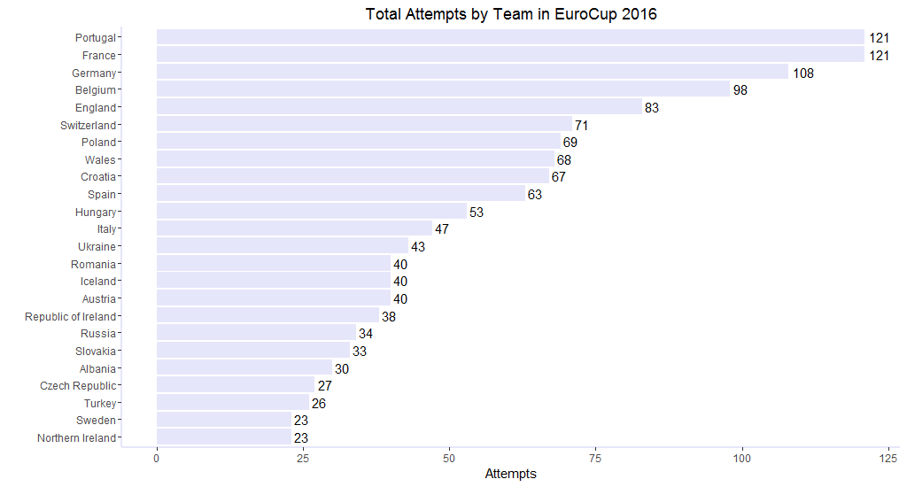
Now I want all the grid lines go.

ggplot(attempts, aes(x = reorder(Name, Total.attempts), y = Total.attempts)) +
  geom_bar(stat = "identity", fill = "lavender") +
  geom_text(aes(label = Total.attempts), hjust = -0.2) +
  coord_flip() +
  ggtitle("Total Attempts by Team in EuroCup 2016") +
  labs(x = "", y = "Attempts") +
  theme(panel.background = element_blank()) ###

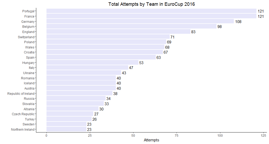
Okay, without the x-axis the plot doesn’t look good to me. So I have added an x-axis line with the same colour as bar.

ggplot(attempts, aes(x = reorder(Name, Total.attempts), y = Total.attempts)) +
  geom_bar(stat = "identity", fill = "lavender") +
  geom_text(aes(label = Total.attempts), hjust = -0.2) +
  coord_flip() +
  ggtitle("Total Attempts by Team in EuroCup 2016") +
  labs(x = "", y = "Attempts") +
  theme(axis.line.x = element_line(size = .8, colour = "lavender"), ###
        panel.background = element_blank())

Or, we can draw lines on both axes.

ggplot(attempts, aes(x = reorder(Name, Total.attempts), y = Total.attempts)) +
  geom_bar(stat = "identity", fill = "lavender") +
  geom_text(aes(label = Total.attempts), hjust = -0.2) +
  coord_flip() +
  ggtitle("Total Attempts by Team in EuroCup 2016") +
  labs(x = "", y = "Attempts") +
  theme(axis.line.x = element_line(size = .8, colour = "lavender"),
        axis.line.y = element_line(size = .8, colour = "lavender"), ###
        panel.background = element_blank())

Or, if we don’t want lavender colour as axes lines.

ggplot(attempts, aes(x = reorder(Name, Total.attempts), y = Total.attempts)) +
  geom_bar(stat = "identity", fill = "lavender") +
  geom_text(aes(label = Total.attempts), hjust = -0.2) +
  coord_flip() +
  ggtitle("Total Attempts by Team in EuroCup 2016") +
  labs(x = "", y = "Attempts") +
  theme(axis.line.x = element_line(size = .8, colour = "black"), ###
        axis.line.y = element_line(size = .8, colour = "black"), ###
        panel.background = element_blank())

However, in a bar plot like this, I prefer to have just one axis line and that is x-axis and in black colour.

ggplot(attempts, aes(x = reorder(Name, Total.attempts), y = Total.attempts)) +
  geom_bar(stat = "identity", fill = "lavender") +
  geom_text(aes(label = Total.attempts), hjust = -0.2) +
  coord_flip() +
  ggtitle("Total Attempts by Team in EuroCup 2016") +
  labs(x = "", y = "Attempts") +
  theme(axis.line.x = element_line(size = .6, colour = "black"), ###
        panel.background = element_blank())

I would also like to use one of my favorite fonts for title and keep the other texts as it is. For that we need to load another package call extrafont. You have to load all the fonts available in your computer first(one time). Check the package detail for more info. Once you are done with the load, you can check the available fonts with fonts() function. I have also increased font size of axes texts and title. One line of code is added in order to run windows font.

windowsFonts(MB=windowsFont("Mongolian Baiti")) ###
ggplot(attempts, aes(x = reorder(Name, Total.attempts), y = Total.attempts)) +
  geom_bar(stat = "identity", fill = "lavender") +
  geom_text(aes(label = Total.attempts), hjust = -0.2) +
  coord_flip() +
  ggtitle("Total Attempts by Team in EuroCup 2016") +
  labs(x = "", y = "Attempts") +
  theme(axis.line.x = element_line(size = .6, colour = "black"),
        axis.text = element_text(size = 11), ###
        axis.title = element_text(size = 11), ###
        panel.background = element_blank(),
        plot.title = element_text(size = 20, family = "Mongolian Baiti")) ###

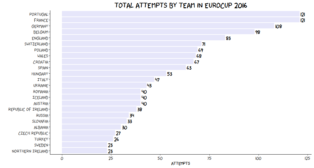
Because of extrafont package we can create XKCD style bar plot by loading xkcd font. Check out more info about XKCD.

windowsFonts(xkcd=windowsFont("xkcd")) ###
ggplot(attempts, aes(x = reorder(Name, Total.attempts), y = Total.attempts)) +
  geom_bar(stat = "identity", fill = "lavender") +
  geom_text(aes(label = Total.attempts, family = "xkcd"), hjust = -0.2) + ###
  coord_flip() +
  ggtitle("Total Attempts by Team in EuroCup 2016") +
  labs(x = "", y = "Attempts") +
  theme(axis.line.x = element_line(size = .6, colour = "black"),
        axis.line.y = element_line(size = .6, colour = "black"), ###
        axis.text = element_text(size = 11),
        axis.title = element_text(size = 11),
        panel.background = element_blank(),
        plot.title = element_text(size = 20, family = "xkcd"), ###
        text = element_text(family = "xkcd")) ###

We can do some popular themes as well like FiveThirtyEight and The Economist, but in order to resemble their bar plots, we need to load some paid fonts which I can’t afford at the moment. So I will leave that out.

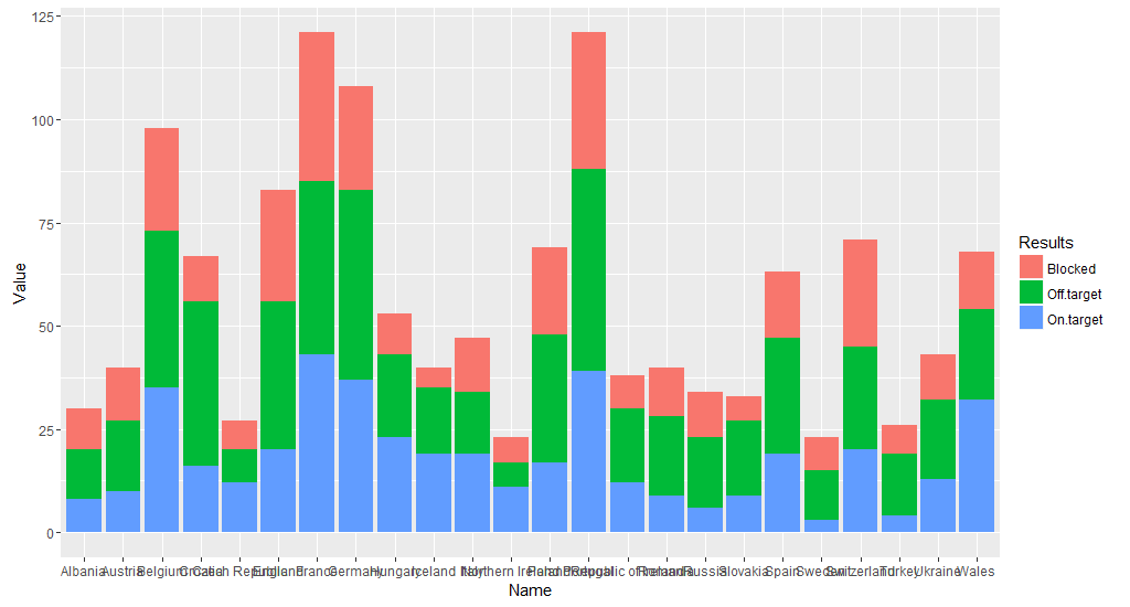
Stacked Bar Plot

Let’s build a stacked bar plot which shows On.target, Off.target, Blocked. For this we need to change to data table into long format with tidyr package.

Select only the variables which is required.

require(tidyr)

attempts <- select(attempts, Name, On.target, Off.target, Blocked)
attempts_long <- gather(attempts, "Result", "Value", 2:4)

Let’s look at the first few lines of the new data.

head(attempts_long)

Name	Results	Value
France	On.target	43
Wales	On.target	32
Portugal	On.target	39
Belgium	On.target	35
Iceland	On.target	19
Germany	On.target	37

So let’s build the first stacked bar plot.

ggplot(attempts_long, aes(x = Name, y = Value, fill = Results)) +
  geom_bar(stat = "identity")

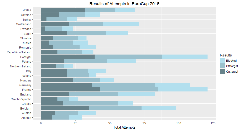
I have added title, y-axis title and left x-axis title as blank, changed the colour of the stacked bar and flipped the plot.

ggplot(attempts_long, aes(x = Name, y = Value, fill = Results)) +
  geom_bar(stat = "identity") +
  ggtitle("Results of Attempts in EuroCup 2016") + ###
  labs(y = "Total Attempts", x = "") + ###
  scale_fill_manual(values = c("lightblue2", "lightblue3", "lightblue4")) + ###
  coord_flip() ###

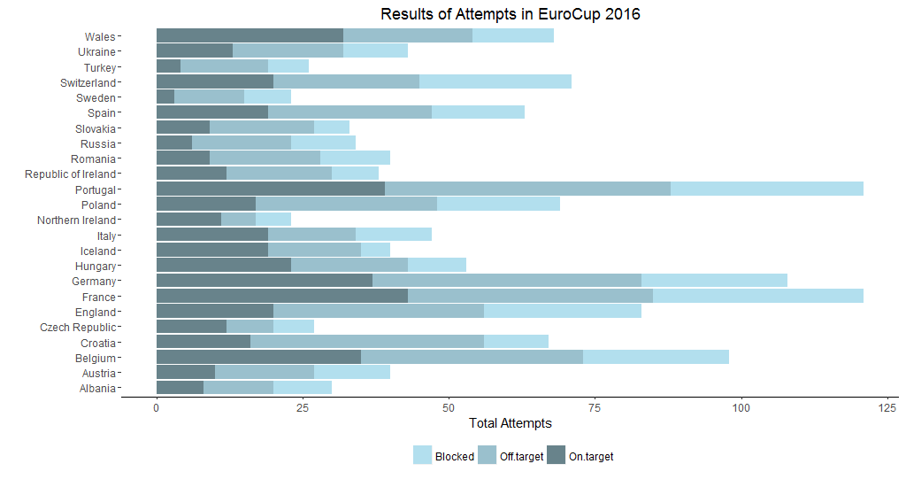
I prefer legend to be at the bottom and make the plot background as white with just horizontal-axis line.

ggplot(attempts_long, aes(x = Name, y = Value, fill = Results)) +
  geom_bar(stat = "identity") +
  ggtitle("Results of Attempts in EuroCup 2016") +
  labs(y = "Total Attempts", x = "") +
  scale_fill_manual(values = c("lightblue2", "lightblue3", "lightblue4")) +
  coord_flip() +
  theme(legend.position = "bottom", legend.direction = "horizontal", ###
        legend.title = element_blank(),  ###
        panel.background = element_blank(), ###
        axis.line.x = element_line(size = .6, colour = "black")) ###

Let’s put the value of each results - On.target, Off.target and Blocked in their respective area of the bar.

ggplot(attempts_long, aes(x = Name, y = Value, fill = Results)) +
  geom_bar(stat = "identity") +
  ggtitle("Results of Attempts in EuroCup 2016") +
  labs(y = "Total Attempts", x = "") +
  scale_fill_manual(values = c("lightblue2", "lightblue3", "lightblue4")) +
  coord_flip() +
  geom_text(aes(label = Value)) + ###
  theme(legend.position = "bottom", legend.direction = "horizontal",
        legend.title = element_blank(),
        panel.background = element_blank(),
        axis.line.x = element_line(size = .6, colour = "black"))

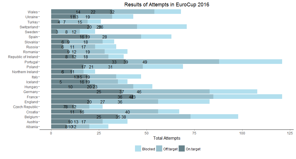
Notice that the values are all dispersed. In order to display the values at the preffered area of the bar, I need to make some changes. We will use ddply() function from plyr package. Create a new variable call pos so that we can place values at the center of their respective area. The code is taken from stackoverflow answer.

new_attempts <- ddply(attempts_long, .(Name), transform,
                   pos = cumsum(Value) - (0.5 * Value))

The new data table looks like this

head(new_attempts)

Name	Results	Value	pos
Albania	On.target	8	4.0
Albania	Off.target	12	14.0
Albania	Blocked	10	25.0
Austria	On.target	10	5.0
Austria	Off.target	17	18.5
Austria	Blocked	13	33.5

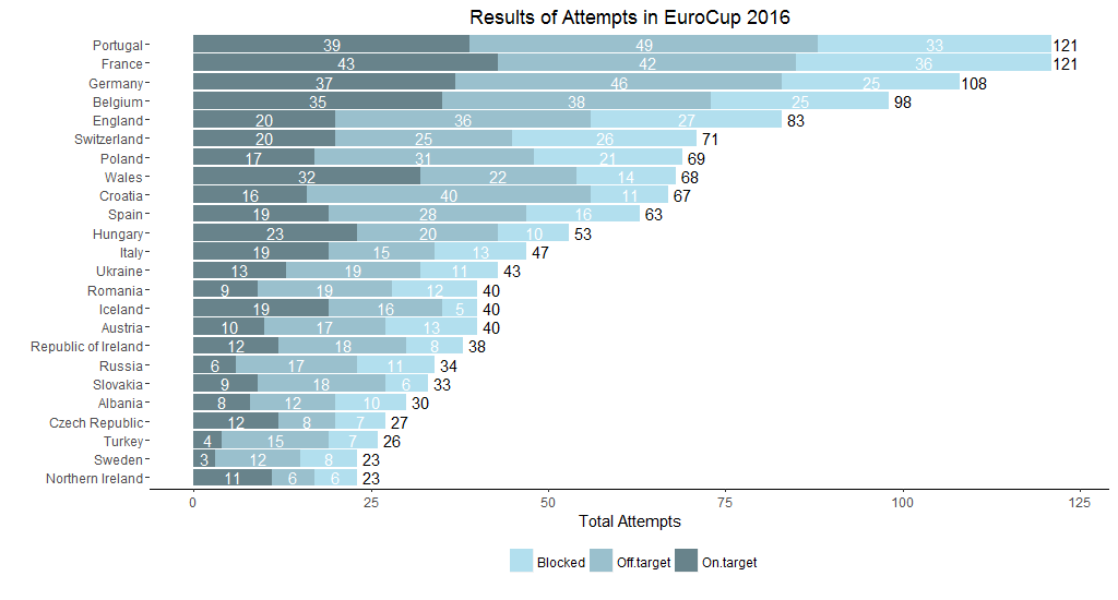
Also change the colour of value into white and size to 4.

ggplot(new_attempts, aes(x = reorder(Name, Value),y = Value ,fill = Results)) +
  geom_bar(stat = "identity") +
  ggtitle("Results of Attempts in EuroCup 2016") +
  labs(y = "Total Attempts", x = "") +
  scale_fill_manual(values = c("lightblue2", "lightblue3", "lightblue4")) +
  coord_flip() +
  geom_text(aes(x = Name, y = pos, label = Value), size = 4, colour = "white") + ###
  theme(legend.position = "bottom", legend.direction = "horizontal",
        legend.title = element_blank(),
        panel.background = element_blank(),
        axis.line.x = element_line(size = .6, colour = "black"))

Now, I want to add the sum value as well on the tip of each bar, similar to the normal bar plot we plotted above. For this I need the variable Total.attempts from original data attempts. However, I have noticed that I have not selected this variable while transforming the data. So I going to recreate this variable.

attempts$Total <- rowSums(attempts[, 2:4])

In order to add the values of Total, I have saved the plot in an object.

attempts_plot <- ggplot(new_attempts, aes(x = reorder(Name, Value),y = Value ,fill = Results)) +
                        geom_bar(stat = "identity") +
                        ggtitle("Results of Attempts in EuroCup 2016") +
                        labs(y = "Total Attempts", x = "") +
                        scale_fill_manual(values = c("lightblue2", "lightblue3", "lightblue4")) +
                        coord_flip() +
                        geom_text(aes(x = Name, y = pos, label = Value), size = 4, colour = "white") +
                        theme(legend.position = "bottom", legend.direction = "horizontal",
                              legend.title = element_blank(),
                              panel.background = element_blank(),
                              axis.line.x = element_line(size = .6, colour = "black"))

and add this code to display the values of Total. This code is derived from stackoverflow answer

attempts_plot +
  geom_text(aes(Name, Total + 2, label = Total, fill = NULL), size = 4, data = attempts) ###

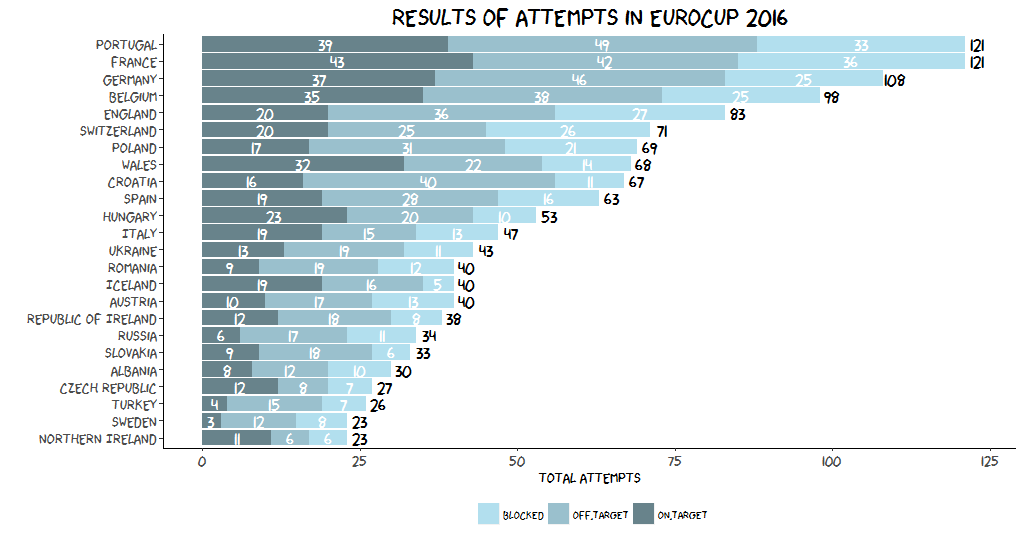
Let me draw the plot with xkcd font.

windowsFonts(xkcd=windowsFont("xkcd")) ###
attempts_xkcd <- ggplot(new_attempts, aes(x = reorder(Name, Value),y = Value ,fill = Results)) +
                        geom_bar(stat = "identity") +
                        ggtitle("Results of Attempts in EuroCup 2016") +
                        labs(y = "Total Attempts", x = "") +
                        scale_fill_manual(values = c("lightblue2", "lightblue3", "lightblue4")) +
                        coord_flip() +
                        geom_text(aes(x = Name, y = pos, label = Value), size = 5, 
                        colour = "white", family = "xkcd") + ###
                        theme(legend.position = "bottom", legend.direction = "horizontal",
                              legend.title = element_blank(),
                              panel.background = element_blank(),
                              axis.line.x = element_line(size = .6, colour = "black"),
                              axis.line.y = element_line(size = .6, colour = "black"),
                              plot.title = element_text(size = 20, family = "xkcd"), ###
                              text = element_text(family = "xkcd"), ###
                              axis.text = element_text(size = 12), ###
                              axis.title = element_text(size = 12)) ###

attempts_xkcd + 
  geom_text(aes(Name, Total + 2, label = Total, fill = NULL),
            family = "xkcd", size = 5, data = attempts) ###

Resources

Thanks for reading out and I hope this helps a bit to construct your bar plot using ggplot2 package smoothly.